Question answered: “How many times higher are the odds of the event in the exposed group?”
Metric = 1.0: No association (exposure does not change the risk/odds).
Metric > 1.0: Harmful exposure (higher risk/odds in the exposed group).
Metric < 1.0: Protective exposure (lower risk/odds in the exposed group).
Cohort study
Cohort
A group of people who share a common characteristic or experience within a defined period of time.
Idea
Select a group of people (cohort)
with shared similar characteristics (Age, sex, etc.)
with different exposures (e.g., smoking vs. non-smoking)
Follow them over time to see who develops the disease of interest (e.g., lung cancer).
Data Source: EHR
Common analytical framework: Logistic regression, machine learning models
Retrospective cohort study
Looking back from the history of the cohort to determine exposure status and outcome.
Find out who were exposed and who were not exposed in the past.
Find out who develops the disease of interest after the exposure.
Illustration of retrospective cohort study
Case control study
We select a group of people with
similar characteristics (e.g., age, sex)
with different disease (e.g., cancer vs. non-cancer),
Check what kind of exposure they had before the disease
Illustration of case-control study
Comparison
Feature
Cohort
Case-Control
Starting Point
Exposure status
Disease status (Outcome)
Direction of Inquiry
Forward (Exposure → Outcome)
Backward (Outcome → Exposure)
Primary Metric
Relative Risk (RR)
Odds Ratio (OR)
Ideal Use Case
Rare exposures
Rare diseases
Can measure incidence?
Yes
No
Workshop: cohort study
Scenario: A suspected outbreak
Presenting issue
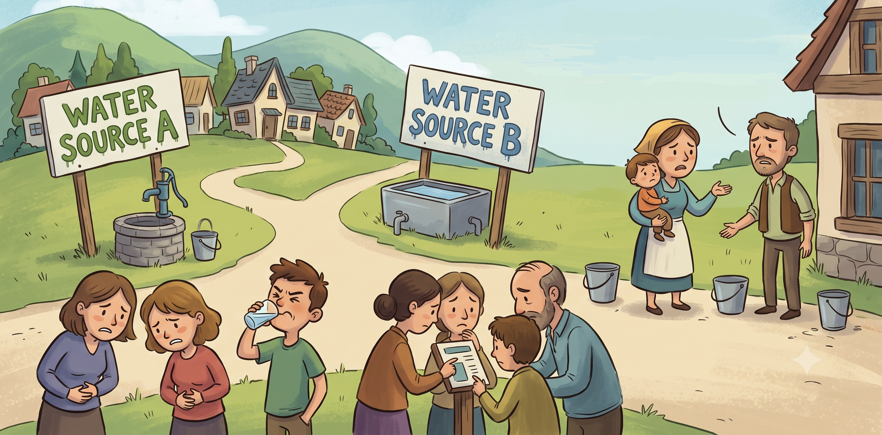
A small community that relies on two drinking-water sources, Water Source A and Water Source B. Several residents develop disease after directly drinking water.
Questions
Investigators want to know whether living near one water source increases the risk of infection.
Illustration
Activity instructions
In a cohort study, we follow a specific population based on their exposure status to observe their future probability of developing a disease.
Everyone in the class: show only the card back (Water Source) and hide the face.
Investigation: leave your seat and find \(N\)residents from Area A and \(N\)residents from Area B.
Once you find them, ask them to reveal their card faces and record whether they are infected (Red card).
Record your data in the table below in R:
Cohort Study
Infected (Red)
Healthy (Black)
Water Source A (Exposed = \(N\))
a
b
Water Source B (Unexposed = \(N\))
c
d
Interpretation of cohort study
The fundamental question we can answer is:
Compared with the unexposed group, how likely is the exposed group to develop the disease (outcome)?
To answer this, we need to know
How likely is the outcome to occur in the unexposed group? (Risk)
How likely is the outcome to occur in the exposed group? (Risk)
Calculate the ratio of 2. to 1. (Relative Risk)
# Enter the data (a, b, c, d) you collected from your Cohort Studya <-15# Number of infected in Area A (example)b <-3# Number of healthy in Area A (example)c <-2# Number of infected in Area B (example)d <-10# Number of healthy in Area B (example)# Calculate the Risk (Incidence)risk_A <- a / (a + b)risk_B <- c / (c + d)# Calculate Relative Risk (RR)RR <- risk_A / risk_Bcat("Relative Risk (RR) of the Cohort Study:", round(RR, 2), "\n")
Relative Risk (RR) of the Cohort Study: 5
Discussion
Current methods is the simplest way to estimate the RR. However, some obvious pitfall includes
Cannot incorporate other control variables (e.g. sex, age, etc …)
Cannot get a confidence interval to perform inference test.
Generalized linear model
Helper function:
Transform contingency table to proper long table with age as confounder
# Expand 2x2 counts into individual patient rowscohort_data <-data.frame(exposure =factor(c(rep("A", a + b), rep("B", c + d)), levels =c("B", "A")),infected =c(rep(1, a), rep(0, b), rep(1, c), rep(0, d)))# Simulate a confounder: older age increases both exposure to A and infection riskset.seed(42)cohort_data$age <-round(rnorm(nrow(cohort_data), mean =45, sd =5) +ifelse(cohort_data$exposure =="A"& cohort_data$infected ==1, 5, 0))head(cohort_data)
  exposure infected age
1        A        1  57
2        A        1  47
3        A        1  52
4        A        1  53
5        A        1  52
6        A        1  49
Poisson Regression (Directly Estimating RR)
Estimate Relative Risk with covariate adjustment through Poisson regression
# Fit Logistic Regression Modellogistic_model <-glm(infected ~ exposure + age, data = cohort_data, family =binomial(link ="logit"))# Extract adjusted OR and 95% CIor_est <-exp(coef(logistic_model)["exposureA"])or_ci <-exp(confint.default(logistic_model)["exposureA", ])summary(logistic_model)
Call:
glm(formula = infected ~ exposure + age, family = binomial(link = "logit"),
    data = cohort_data)

Coefficients:
            Estimate Std. Error z value Pr(>|z|)
(Intercept)  -8.1736     4.0678  -2.009  0.04450 *
exposureA     2.7570     1.0679   2.582  0.00983 **
age           0.1442     0.0846   1.704  0.08838 .
---
Signif. codes:  0 '***' 0.001 '**' 0.01 '*' 0.05 '.' 0.1 ' ' 1

(Dispersion parameter for binomial family taken to be 1)

    Null deviance: 41.054  on 29  degrees of freedom
Residual deviance: 23.530  on 27  degrees of freedom
AIC: 29.53

Number of Fisher Scoring iterations: 5
Relative Risk (RR):\[
\small
RR = \frac{\text{Risk in Exposed}}{\text{Risk in Unexposed}} = \frac{\frac{a}{a+b}}{\frac{c}{c+d}}
\]
Odds Ratio (OR):
\[
\small
OR = \frac{\text{Odds in Exposed}}{\text{Odds in Unexposed}} = \frac{\frac{a}{b}}{\frac{c}{d}} = \frac{a \times d}{b \times c}
\]
If a disease is extremely rare (e.g., 1 in 10,000 people), the number of sick (\(a\) and \(c\)) is incredibly tiny compared to the healthy people (\(b\) and \(d\)).
If \(a\) is vanishingly small, then adding it to \(b\) barely changes anything. Therefore the following approximation holds \[
\small
\begin{aligned}
a \ll b \implies & a + b \approx b \\
c \ll d \implies & c + d \approx d
\end{aligned}
\]
Summary
Context
Recommend methods
Why?
Outcome is Rare (\(<5\% - 10\%\))
Logistic Regression
\(\text{OR} \approx \text{RR}\); computation is fast, robust, and universally accepted.
Outcome is Common (\(>10\%\)) in a Cohort
Poisson Regression
Directly yields an interpretable Relative Risk without exaggerating effect size.
Prediction Modeling / Risk Calculators / Case control study
Logistic Regression
Guaranteed to bound individual risk estimates within \([0, 1]\).